July 27, 2026

Inventory Control For Small And Medium Companies

Why Inventory Optimization Analytics Matter for SMEs

For small and medium-sized enterprises that hold physical stock — whether it’s raw materials, spare parts, or finished goods — inventory is usually one of the largest tied-up assets on the balance sheet. Get it wrong in one direction and you’re sitting on cash that’s frozen in stock nobody’s buying. Get it wrong in the other direction and you’re missing sales, disappointing customers, or paying rush-shipping premiums because you ran out of something at the worst possible moment.

This is a genuinely hard balancing act, and it’s usually a bigger problem for SMEs than for large enterprises, not a smaller one. A large retailer can absorb a badly-stocked SKU across thousands of others. An SME with a few hundred SKUs and a tight cash position feels every misjudged reorder directly — either in warehouse rent for stock that isn’t moving, or in lost sales when a supplier’s six-week lead time turns into a stockout.

The traditional way this gets handled at a small business is gut feel: “we always order 100 of these,” “let’s reorder when it looks low,” “call the supplier again, we’re running low on the popular one.” That works, until the business grows past the point where one person can hold the whole inventory picture in their head — and by then, the cost of getting it wrong has grown right along with it.

This is where inventory optimization analytics comes in: a set of well-established, decades-old formulas — ABC analysis, Economic Order Quantity, safety stock, and reorder points — that replace “gut feel” with a number for how much to order, when, and for which items it’s worth paying the closest attention to. None of this requires enterprise software or a data science team. It requires knowing your costs, demand, and lead times per item, and running some fairly simple math against them.

What inventory optimization analytics actually gives you

Benefit	Why it matters for SMEs
Frees up cash	Right-sized order quantities and reorder points mean less capital sitting in excess stock.
Reduces stockouts	Reorder points built from actual demand variability and supplier lead time catch shortages before they happen — not after.
Focuses limited attention	ABC analysis tells you which 20% of SKUs drive 80% of your inventory value, so scarce management time goes where it matters most.
Lowers ordering & holding costs together	EOQ finds the order quantity that minimizes the combined cost of placing orders and holding stock — not just one or the other.
Builds in a safety margin, deliberately	Safety stock is sized to a chosen service level, so the buffer against demand spikes or late deliveries is a decision, not an accident.
Enables forecasting and budgeting	Knowing reorder points and order quantities per SKU turns “we might need to order soon” into a plannable, budgetable cash outflow.
Supports data-driven purchasing decisions	Replaces “we’ve always ordered this much” with numbers grounded in actual cost, demand, and lead-time data.

For a cash-constrained SME, the first two rows are usually the ones that matter most: money tied up in the wrong stock is money that can’t be spent on marketing, hiring, or simply staying solvent through a slow month — and a stockout on a top-selling item can lose a customer for good.

A practical example

Let’s use a fictitious example. Say an SME distributes hardware components and carries 200 different SKUs. Without any analysis, every SKU gets treated more or less the same: the warehouse manager reorders “the usual amount” whenever stock looks low, for every item, regardless of how much money is actually tied up in it.

With ABC analysis, the same 200 SKUs get sorted by annual consumption value (annual demand × unit cost) and classified by how much of the total value they represent:

Class	Items	% of SKUs	% of Consumption Value
A	94	49.5%	79.9%
B	46	24.2%	15.1%
C	50	26.3%	5.0%

The insight: roughly half the SKUs (Class A) account for nearly 80% of the money tied up in inventory. That’s exactly where a warehouse manager’s attention should go first — tighter monitoring, more frequent reviews, closer supplier relationships — while the Class C tail (a quarter of value, spread across a similar number of items) can be managed with looser, less time-consuming rules. Nobody needs to spend the same amount of care reviewing a $50/year fastener as a $2,000,000/year electronics component.

More precise numbers, per SKU

Once you know which SKUs deserve attention, the next question is how much to order and when. That’s where the per-item formulas come in:

• Economic Order Quantity (EOQ) answers “how much should we order at once?” by balancing the fixed cost of placing an order against the cost of holding stock — order too little and you pay ordering costs constantly; order too much and holding costs eat the savings.
• Safety stock answers “how much buffer do we need?” based on how variable daily demand is and how long the supplier takes to deliver, tuned to a target service level (e.g. 95% or 99% of demand covered without stockout).
• Reorder point (ROP) answers “at what stock level do we place the next order?” — expected demand during the lead time, plus that safety buffer.
• Min/Max levels give simple operational thresholds: reorder at Min (the reorder point), order up to Max (reorder point + EOQ).

Two SKUs with similar sales volume can need very different reorder behavior if one has a 3-day lead time and steady demand, and the other has a 60-day lead time and volatile demand — the formulas capture that automatically, instead of relying on the same rule of thumb for both.

The business impact, in real numbers

Consider an SME with 200 SKUs and roughly $1M tied up in average inventory, with excess safety margins on most items because reorder decisions have always been made by eyeballing stock levels.

If inventory optimization analytics reveals that a meaningful share of Class B and C items are carrying far more safety stock than their actual demand variability and lead time justify — even a 10% reduction in excess stock across those items frees up real cash: on $1M in average inventory, that’s $100,000 back on the balance sheet, without cutting a single SKU or changing what’s offered to customers.

At the same time, tightening reorder points on the Class A items that actually drive revenue — rather than treating them the same as everything else — reduces the chance of a stockout on the products that matter most, protecting the sales those items were already generating.

That’s the core case for inventory optimization: it very often frees up cash and reduces stockout risk at the same time, by pointing the same amount of purchasing effort at the items where it actually pays off.

Try it yourself: a demo you can run in minutes

To make these concepts concrete, this repository — Inventory-Control — is a small open-source demo. It’s a Python-based pipeline that:

1. Generates a batch of synthetic (fake) SKUs — cost, demand, lead time, current stock, supplier, category, etc.
2. Validates that data against a strict set of business rules.
3. Runs the standard inventory-optimization formulas described above — ABC class, EOQ, safety stock, reorder point, and max level — per SKU.
4. Produces an Excel workbook with the input data, the full analysis results, and an ABC summary sheet — the same kind of view described above, generated automatically.

It’s designed as a learning and demonstration tool, so you can see how ABC/EOQ/safety stock logic works end-to-end without connecting it to a real ERP or warehouse system. The math itself follows the standard methods described on abcsupplychain.com’s inventory management articles.

Downloading the code (no Git experience needed)

Just download the code from the Github repository, and ask your AI tool of choice (I used Claude) to generate a Python environment and the dependencies listed in requirements.txt. Then run analysis.py. Even if you want to do everything yourself, you don’t need to know Git or the command line to get the code onto your computer:

1. Go to the repository: github.com/MattProtopapas/Inventory-Control-Demo
2. Click the green <> Code button near the top of the page.
3. In the dropdown, click “Download ZIP”.
4. Once downloaded, right-click the ZIP file and choose “Extract All…“ (Windows) to unzip it into a regular folder.
5. Open that extracted folder — that’s the project.

If you’re comfortable with Git, git clone https://github.com/MattProtopapas/Inventory-Control-Demo.git does the same thing in one step — but the ZIP download works just as well and requires no tools beyond what’s already built into Windows.

Running the demo

The project includes a requirements.txt file and a full README.md, but the short version is:

1. Install Python 3.10 or higher, if you don’t already have it, from python.org — the pipeline uses statistics.NormalDist and modern type hints, so it needs 3.10+, but in exchange it needs no numpy or scipy.
2. Open the extracted folder in a terminal (PowerShell on Windows) and create a virtual environment:

   python -m venv .venv
   .venv\Scripts\Activate.ps1
   

3. Install the dependencies:

   pip install -r requirements.txt
   

4. Run the three pipeline steps in order:

   python generate_data.py --count 200 --error-rate 0.05 --seed 42
   python validate_data.py
   python analyze_inventory.py
   

Running these three scripts will:

• Generate a synthetic inventory dataset (data/inventory_raw.csv) — with a small, configurable share of rows deliberately corrupted (negative costs, blank fields, an out-of-range service level, a duplicate SKU) so the next step has real errors to catch.
• Validate that data, dropping anything invalid or duplicated, and write the clean rows to data/inventory_validated.csv plus a plain-text explanation of every rejection to data/validation_report.txt.
• Compute EOQ, safety stock, reorder point, max level, and ABC class per SKU, and produce output/inventory_analysis.xlsx.

Open that Excel file afterward to see the same kind of ABC breakdown and reorder logic described earlier in this post, calculated on the data you just generated. You can rerun generate_data.py with a different --count, --error-rate, or --seed to see how the results change with a different dataset — a useful way to build intuition for how ABC splits and reorder points respond to different demand and cost profiles.

Every script also accepts custom --input/--output paths, so once you’re comfortable with the demo you can point validate_data.py straight at a real inventory export (matching the columns in inventory_common.py) and skip generate_data.py entirely, running your own numbers through the same validation and analysis steps.

Note: this demo uses synthetic, randomly generated data and is intended for educational and demonstration purposes only — see the repository’s Disclaimer & EULA for details. It’s a starting point for understanding the mechanics of ABC/EOQ/safety stock analysis, not a production-ready inventory management system.

Understanding the results

inventory_analysis.xlsx has three sheets, and each one represents a stage of the analysis described earlier in this post — from raw SKU data down to a prioritized, per-item action list.

Sheet 1: Input Data

This is the raw material: one row per SKU, with fields like SKU, item name, category, supplier, warehouse location, unit cost, annual demand, daily demand standard deviation, lead time, current stock, ordering cost, holding cost percentage, target service level, and last restock date — exactly the validated rows the analysis was run on.

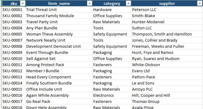
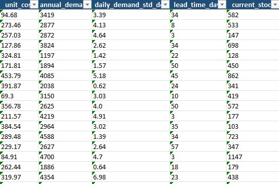
In this demo, the data is entirely synthetic — generated by generate_data.py, not pulled from a real ERP or warehouse system. That’s deliberate: it keeps the demo self-contained and lets you see validation actually catch problems (a configurable percentage of rows are deliberately corrupted with negative costs, blank fields, and an out-of-range service level). An SME that wants to see their own numbers would replace this generation step with an export from their inventory system or spreadsheet (same column structure), and everything downstream would run exactly the same way.

Sheet 2: Analysis Results

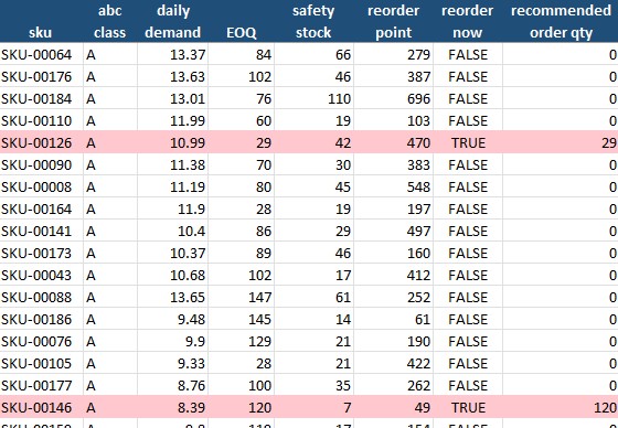
This is where the per-SKU math lands: ABC class, annual consumption value, daily demand, EOQ, safety stock, reorder point, max level, current stock, whether the item needs reordering right now, and the recommended order quantity if so. Rows sorted by consumption value, with any SKU at or below its reorder point highlighted in red so it’s immediately visible without having to scan every row.

Reading a couple of rows from the sample above: SKU-00126 (“Happy Shoulder Component,” an Electronics item) is Class A, sitting at 214 units of current stock against a reorder point of 470 — it’s flagged TRUE for reorder, with a recommended order of 29 units (its EOQ). Just above it, SKU-00184 (“Most Animal Bundle,” Hardware) is also Class A but sitting comfortably above its reorder point at 973 units against a threshold of 696 — no action needed yet. That’s the entire point of the sheet: instead of checking every SKU manually, the highlighted rows tell a purchasing manager exactly which items need attention today.

Sheet 3: ABC Summary

The last sheet rolls the per-SKU detail up into the view a manager actually needs for prioritization: item count, percentage of items, total consumption value, percentage of value, and how many items in each class currently need reordering, broken out by A/B/C class.

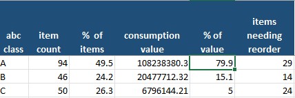
• Class A (94 items, 49.5% of SKUs) accounts for 79.9% of total consumption value, with 29 items currently needing reorder. This is the class deserving the tightest monitoring and the fastest supplier relationships — it’s where nearly four-fifths of the inventory investment lives.
• Class B (46 items, 24.2% of SKUs) accounts for 15.1% of value, with 14 items needing reorder — worth periodic review, but not the same intensity as Class A.
• Class C (50 items, 26.3% of SKUs) accounts for just 5.0% of value, with 24 items needing reorder. Even though nearly as many Class C items need reordering as Class A, each one represents far less capital at risk — these can typically be handled with simple, low-effort reorder rules (or even bulk, infrequent restocking) without much oversight.

Of course those results by themselves do not provide a holistic approach in inventory control managment. This kind of analyses however, what a larger company might do, when customized for a company’s specific decision patterns and available data, are the ones that can lead to a sound inventory management strategy that optimizes costs, while accounting for an appropriate level of customer service.

← Back to all posts