Every SME owner and individual investor eventually ends up holding more than one asset — a mix of stocks, bonds, cash reserves, maybe a rental property or a stake in another business. The usual way that mix gets decided is gut feel: “I’ll put most of it in something safe, a bit in something that might grow, and diversify a little just in case.” That instinct isn’t wrong, but it’s also not a number. It doesn’t say how much risk that mix carries, whether a different split would have earned more for the same risk, or whether one of the holdings is quietly doing nothing for the portfolio at all.
Previous posts on this blog have made the same argument for sales data and stock data: replace gut feel with a number, using data that’s already available. Markowitz Mean-Variance Optimization (MVO) — the Nobel Prize-winning framework behind modern portfolio theory, dating back to Harry Markowitz’s 1952 paper — does exactly that for investment allocation. Instead of asking “does this feel diversified,” it asks “for every unit of risk taken on, is this the best possible expected return available from this set of assets” — and answers it with a precise, repeatable calculation instead of an impression.
What Markowitz portfolio optimization actually gives you
| Benefit | Why it matters for SMEs and individual investors |
|---|---|
| Quantifies the risk/return trade-off | Turns “this feels risky” into an actual number — expected return and volatility for any given mix of assets — instead of an impression. |
| Proves diversification instead of assuming it | Combining assets that don’t move in lockstep reduces portfolio risk below the average of the individual assets’ risk — MVO calculates exactly how much, using the covariance between every pair of assets, not just how many different things you hold. |
| Finds the efficient frontier | For any level of risk you’re willing to take, there’s a mix of assets that maximizes expected return — and a mix that doesn’t. The frontier shows you which one you’re holding. |
| Flags assets that aren’t earning their place | If an asset doesn’t improve the risk/return trade-off of the whole portfolio, the optimizer assigns it zero weight — a concrete, evidence-based reason to hold it or drop it, rather than “it’s always been in there.” |
| Enforces constraints you actually care about | Long-only, a maximum weight per position, no short-selling — real limits (regulatory, risk-appetite, or just personal comfort) can be built directly into the optimization instead of applied by eye afterward. |
| Makes estimation risk visible | Comparing the return you expect to the return your data actually shows — see below — surfaces how much of that expectation is signal versus noise, before money moves on the strength of it. |
For an SME managing surplus cash or a reserve fund, or an individual investor managing personal savings, the second and third rows are usually where the most value is hiding: most gut-feel portfolios are already diversified in the naive sense (multiple asset classes) but not in the mathematical sense (low or negative correlation between them) — and that gap is exactly what this framework is built to close.
A practical example, using this repo’s own results
This repository — Markowitz-Portfolio-Optimization-Demo — ships with a full worked example rather than a hypothetical one. Running it with the defaults simulates 8 synthetic assets over 756 trading days (about 3 years of daily prices), deliberately corrupts about 1% of the return data to test the pipeline, then validates, optimizes, and reports the results.
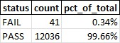
Before anything is optimized, every single observation is checked: 6,048 daily prices (all pass — prices are reconstructed from clean returns, so they’re always valid) and 6,029 daily returns, of which 41 (0.68%) fail validation — implausible one-day moves and missing values, injected on purpose — and are automatically excluded before the expected returns and covariance matrix are estimated. Across both checks combined, that’s 12,077 observations checked, 99.66% passing. This mirrors exactly the role the Data Quality tab played in the market basket analysis demo: catch bad data before it silently distorts the model, rather than after.
The numbers that make this trustworthy — and the honesty of the ones that don’t
With clean data in hand, the pipeline estimates each asset’s annualized expected return and volatility from the sample of daily returns — exactly as you would with real historical price data.
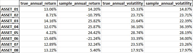
This tab is arguably the most important one in the whole workbook, because it shows both the true parameters used to generate the data and the sample parameters actually estimated from it — something you’d never get to see with real market data, where the “true” expected return is unknowable. The gap between the two columns is the whole point:
- ASSET_06 was generated with a true annual return of 15.68% — one of the best in the universe — but its sample return, estimated from three years of simulated daily data, comes out at -21.24%. A three-year backward-looking window said this was one of the worst assets to hold, when it was actually one of the best.
- ASSET_02 shows the same pattern in miniature: true return 8.71%, sample return -10.79%.
- ASSET_05 swings the other way — a true return of just 4.22%, but a sample return of 24.42%, making a mediocre asset look like a star.
None of this is a bug in the demo; it’s the point the README is explicit about: with realistic annual volatility (15-36% here) and only a few years of daily history, the sample mean is a genuinely noisy estimate of the true mean. This is a well-documented, real critique of naive mean-variance optimization, sometimes called “estimation-error maximization” — feed the optimizer noisy inputs and it will confidently build a portfolio around the noise. It’s a reason to be careful with a short return history, not a reason to distrust the framework itself.
The efficient frontier, and two portfolios worth knowing by name
Once expected returns and the covariance matrix are estimated, the optimizer traces the efficient frontier — for a grid of target returns, the minimum possible volatility achievable at each one — and marks two specific portfolios on it:
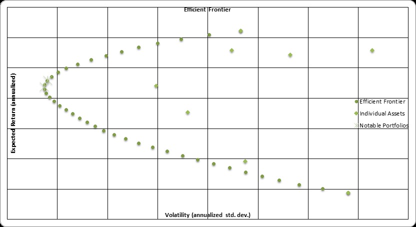
- Global Minimum Variance (GMV) — the single point on the frontier with the lowest possible risk, full stop, regardless of return.
- Maximum Sharpe Ratio — the point that maximizes risk-adjusted return:
(expected
return − risk-free rate) ÷ volatility
. This is usually the more useful reference point, because it answers “which mix gets the most return per unit of risk,” not just “which mix is safest.”
Every diamond on the chart above is a single asset held on its own; every dot along the curve is a diversified combination. The chart makes the core promise of Markowitz’s framework visible at a glance: every individual asset sits below and to the right of the frontier — for the same risk as any single asset, some combination of the full set does better, and for the same return, some combination does it more safely. That gap between “one asset” and “the frontier” is the value diversification adds, made visible instead of assumed.
The business impact, in real numbers
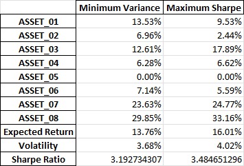
Reading the two portfolios side by side:
| Minimum Variance | Maximum Sharpe | |
|---|---|---|
| Expected return | 13.76% | 16.01% |
| Volatility | 3.68% | 4.02% |
| Sharpe ratio | 3.19 | 3.48 |
Moving from the safest possible portfolio to the Maximum Sharpe portfolio costs 0.34 percentage points of extra volatility and buys 2.25 percentage points of extra expected return — a trade most investors would take without hesitation, and one that’s only visible because the whole frontier was mapped rather than a single “safe” allocation picked by feel.
The weights are just as informative as the headline numbers. ASSET_05 — despite having the fourth-highest sample return out of all 8 assets (24.42%, from the table above, ahead of half the universe) — gets a weight of exactly 0% in both portfolios. On its own that number looks like a screening error; it isn’t. What matters to a mean-variance optimizer isn’t an asset’s return in isolation, it’s the return it contributes net of the risk it adds and the diversification it takes away — and ASSET_05’s volatility and correlation with the rest of the universe make it a net drag on the portfolio despite the attractive headline number. That’s a genuinely counter-intuitive, easy-to-miss conclusion that gut-feel allocation — which tends to chase the asset with the best recent return — would almost certainly get wrong.
What to actually do with this, this week
- Pull 2-3+ years of daily (or weekly) return history for the assets or funds you’re actually choosing between — a brokerage export or a public price API both work.
- Run it through this repo’s pipeline (or a similar tool), swapping the synthetic data
generator for your real return series —
optimization.pyandreport.pydon’t care where the numbers came from. - Check the Validation Summary tab first, before looking at anything else. Bad ticks in a real feed are more common than they look, and they skew a covariance matrix badly if they slip through.
- On the Asset Statistics tab, treat a very high sample return with suspicion, especially over a short history — it’s exactly the pattern that produced ASSET_05’s counter-intuitive zero weight above.
- Pick a point on the Efficient Frontier, not necessarily Max-Sharpe by default — the right point depends on how much volatility you can actually tolerate, which is a personal or business constraint the optimizer doesn’t know on its own.
- Re-run this periodically. Expected returns and correlations both drift; a frontier built on last year’s data is a snapshot, not a permanent allocation.
Try it yourself: a demo you can run in minutes
To make this concrete, this repository — Markowitz-Portfolio-Optimization-Demo — is a small, self-contained, open-source demo. It:
- Generates (or accepts your own) asset price/return data.
- Validates every single observation against pydantic schemas — out-of-range returns, non-positive prices, missing values — so bad source data is caught and dropped with a clear report, rather than silently corrupting the results.
- Solves three classic Markowitz problems with
scipy.optimize.minimize: Global Minimum Variance, Maximum Sharpe Ratio, and the full Efficient Frontier. - Writes everything — inputs, validation logs, asset statistics, the covariance matrix, and both optimal portfolios — into a single Excel workbook, complete with a frontier chart.
Downloading the code (no Git experience needed)
You don’t need to know Git or the command line to get the code onto your computer:
- Go to the repository: github.com/MattProtopapas/Markowitz-Portfolio-Optimization-Demo
- Click the green
<> Codebutton near the top of the page. - Click “Download ZIP” in the dropdown.
- Right-click the downloaded ZIP and choose “Extract All…“ to unzip it into a regular folder.
- Open that folder — that’s the project. Ask your AI tool of choice (I used Claude) to
set up a Python environment and install the dependencies listed in
requirements.txt— no coding experience required to get it running.
If you’re comfortable with Git,
git clone https://github.com/MattProtopapas/Markowitz-Portfolio-Optimization-Demo.git
does the same thing in one step.
Running the demo
The repository includes a full README.md, but the short version, from PowerShell:
python -m venv .venv
.\.venv\Scripts\Activate.ps1
pip install -r requirements.txt

python main.py
That default run generates 8 synthetic assets over ~3 years of daily data and writes
output/mvo_demo_report.xlsx. A handful of CLI options let you reshape the problem
without touching any code:
| Flag | Default | Description |
|---|---|---|
--n-assets |
8 |
Number of synthetic assets |
--n-days |
756 |
Number of simulated trading days |
--risk-free-rate |
0.02 |
Annual risk-free rate used in the Sharpe ratio |
--allow-short-selling |
off | Allow negative portfolio weights |
--max-weight |
1.0 |
Maximum absolute weight per asset — useful for enforcing a concentration limit |
--output |
output/mvo_demo_report.xlsx |
Output workbook path |
For example, a more tightly constrained 12-asset universe:
python main.py --n-assets 12 --max-weight 0.25 --output output/demo_12assets.xlsx
Note: the data generated by this demo is synthetic and randomly generated, and this project is intended for educational and demonstration purposes only — it is not financial advice, and no investment decision should be based solely on its output. See the repository’s Disclaimer & EULA for details. It’s a starting point for understanding how mean-variance optimization works, not a production investment tool.
Understanding the results
output/mvo_demo_report.xlsx has ten tabs, each one a stage of the pipeline described
above: Config, Synthetic Prices, Synthetic Returns, Validation Summary,
Validation Log - Prices, Validation Log - Returns, Asset Statistics, Covariance
Matrix, Efficient Frontier, and Optimal Portfolios — the four screenshots earlier in
this post are pulled directly from the Validation Summary, Asset Statistics,
Efficient Frontier, and Optimal Portfolios tabs, in that order.
The limits worth keeping in mind
Markowitz portfolio optimization, like the market basket and inventory tools covered in earlier posts, is a genuinely useful framework with real limits — and this project is upfront about them rather than hiding them:
- It’s only as good as the inputs. Expected returns estimated from a short history are noisy, as the true-vs-sample gap on the Asset Statistics tab shows directly. This demo deliberately skips shrinkage techniques (Ledoit-Wolf covariance shrinkage, Black-Litterman priors) that real-world practitioners use to dampen that noise — a documented next step, not an oversight.
- It assumes the past is informative about the future — the same limitation that applies to the market basket rules or inventory reorder points covered previously. Correlations and volatilities regimes shift; a frontier from last year isn’t necessarily this year’s frontier.
- It optimizes for variance, not for every risk that matters. Liquidity risk, tail risk, and business-specific cash-flow needs aren’t in the objective function and need separate judgment.
- This is a demonstration, not investment advice. The output is a structured way to think about a trade-off between return and risk using a given set of numbers — it isn’t a recommendation about what to actually buy.
None of that makes the exercise less worthwhile. It just means the output of an optimization run is an input to an investment decision, not the decision itself — in the same way the market basket rules and inventory reorder points from earlier posts are inputs to a merchandising or purchasing decision, not a replacement for judgment. Used that way, Markowitz optimization turns “I think this mix feels diversified” into “I know exactly how much risk and return this mix carries, and what a better combination would look like” — a genuinely useful upgrade for an SME’s treasury reserves or an individual investor’s savings, using nothing more than the same historical price data already sitting in a brokerage statement.