October 5, 2026

How Can A Small Business Forecast Demand For Next Month

Ask the person who places the purchase orders at a small retailer or wholesaler how much of each product they will sell next month and the answer is usually based on gut feeling: “about the same as last month,” “a bit more, it’s coming up to Christmas,” “we always do well on that one in October.” Sometimes the feeling is right. But the order goes in weeks before the sales happen, the supplier’s lead time is fixed, and every unit the feeling gets wrong becomes either a stockout or a pallet of stock that sits in the warehouse until spring.

Every inventory post on this blog so far has quietly assumed demand was known. The reorder points and safety stock post asked how much to order and when; the working capital post asked how much cash it is reasonable to freeze in stock; the OTIF post found stockouts were the single largest cause of failed deliveries. All three start from a number for expected demand. This post is about where that number comes from. Demand forecasting — three textbook methods, an honest way of scoring them, and a direct link from forecast error to safety stock — turns “about the same as last month” into “SKU-001 will sell 1,913 units in the next four weeks, our best method has been wrong by 11.7% on average, and that error means we need 223 units of safety stock rather than 281.”

For a small or medium-sized company, this matters more than the sophistication of the methods suggests. A large retailer has a demand-planning team and software that costs more than an SME’s entire IT budget. An SME has a spreadsheet of weekly sales and one person who knows the products. The good news is that for most products the simple methods get most of the achievable accuracy, and the more useful output is not the forecast itself but the measurement of how wrong it is: which products are predictable enough to order on autopilot, which need a human to look at them, and how much buffer stock each one really needs.

The traditional way this gets handled at a small company is reactive: order what sold last month, add a bit if it feels busy, and fix the stockouts with expedited orders when they happen. What’s missing is the same thing that was missing in the earlier posts — a number, per product, with a stated accuracy, that says what will sell, how sure you can be, and what that uncertainty should cost in safety stock.

What demand forecasting actually gives you

Benefit	Why it matters for an SME
A forecast per product, not a hunch per person	Three methods — seasonal naive, moving average and Holt-Winters exponential smoothing — each turn a weekly sales history into a forecast for the coming weeks. None needs anything beyond the sales figures the business already has.
A fair test of how good each method is	The last quarter of history is held back and never shown to the methods. Each one forecasts it blind and is scored on what actually happened. That is the only honest way to find out whether a method works on your data, rather than in a textbook.
An error you can plan with	MAE (how many units wrong, on average), MAPE (how many percent wrong) and RMSE (the same, but penalising the big misses) turn “the forecast is roughly right” into “this forecast is wrong by 12% in a typical week.”
Catches the systematic mistake	Bias — the signed average error — tells you whether a method consistently over- or under-forecasts. A method can post a respectable MAPE and still make you over-order every single week.
Sorts products into forecastable and not	Banding SKUs by their best achievable error (Easy / Moderate / Hard) tells you which products can be ordered from the forecast and which need judgement, more buffer, or a different approach.
Feeds the inventory numbers directly	Safety stock is z × forecast error × √lead time. A forecast that captures the seasonality has a smaller error than the raw week-to-week swing in demand, so the safety stock it implies is lower — that is the cash a forecast buys you.
Bad data never reaches the forecast	A validation layer rejects negative sales, impossible dates, unknown product codes and duplicate weeks with a stated reason, and reports how many weeks it had to fill in, so nobody mistakes an interpolated value for a real one.

A practical example, using this repo’s own results

This repository — simple-demand-forecasting — ships with a full worked example. The scenario is a fictitious small distributor of consumer goods — beverages, snacks, personal care, pet supplies, garden, toys and stationery — with 30 SKUs and three years (156 weeks) of weekly sales. Each SKU’s demand is built the way real demand behaves: a base level, a gentle trend, a yearly seasonal wave, for some products an extra Q4 peak, occasional promotion weeks with a 1.6–3× lift, and noise. Roughly one product in eight is a slow, lumpy mover selling a handful of units a week. And, as in the earlier demos, a small percentage of rows are deliberately corrupted so the validation step has something real to catch.

The raw sales file has 4,681 rows. The validator rejected 95 of them (2.0%), each with a stated reason: dates that don’t exist (2024-11-99), negative unit sales, unit sales that aren’t numbers, blank or unknown SKU codes (the master has no SKU-999), a promotion flag of “maybe”, and one duplicated SKU-week. Because a weekly series with holes in it can’t be forecast, the 94 weeks that belonged to real SKUs were filled by linear interpolation between their neighbours — and the number of filled weeks is reported per SKU in the league table, so a product whose history is partly made up is labelled as such. What remained is what every forecast in the workbook ran on:

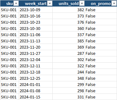
The pipeline then held back the last 13 weeks (6 July – 28 September 2026), fitted all three methods on the first 143 weeks, forecast the holdout blind, and scored the result. The roll-up looks like this:

Read across, the sheet answers the question an SME owner actually has — can I trust this? — before anyone opens the detailed tabs:

• Three SKUs (10%) are Easy: the best method was within 15% of actual sales in a typical week — 9.1% on average. These can be ordered from the forecast.
• Eighteen SKUs (60%), carrying 61% of the unit volume, are Moderate: 15–30% error, 22.3% on average. Good enough to order from with a sensible safety stock, which is exactly what the next-month tab computes.
• Nine SKUs (30%), carrying 24% of the volume, are Hard: more than 30% error, 40.2% on average. The forecast is a starting point for these, not an answer.
• No single method wins. Holt-Winters won 15 SKUs, the moving average 12, and the seasonal naive 3. Had the demo used Holt-Winters for everything, the average error across all 30 SKUs would have been 32.3%; the moving average for everything, 36.8%; picking the best method per SKU brings it down to 26.3%. The most sophisticated method is the best one less than half the time.

Which method, for which product: the league table

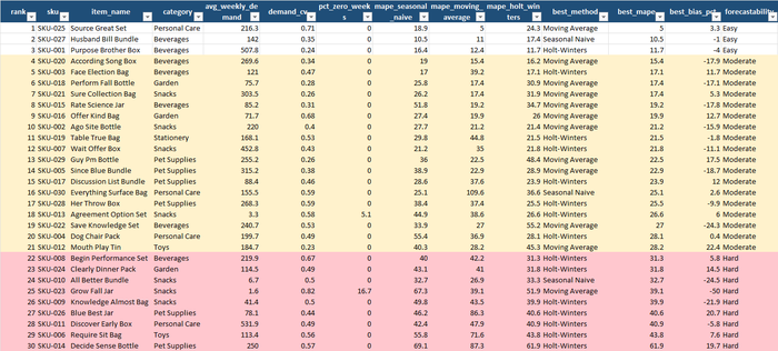
The table is sorted from most to least forecastable, with the Moderate band shaded yellow and the Hard band red. Three columns in the middle show what each method would have scored on the same 13 weeks, and that is where the useful lessons are:

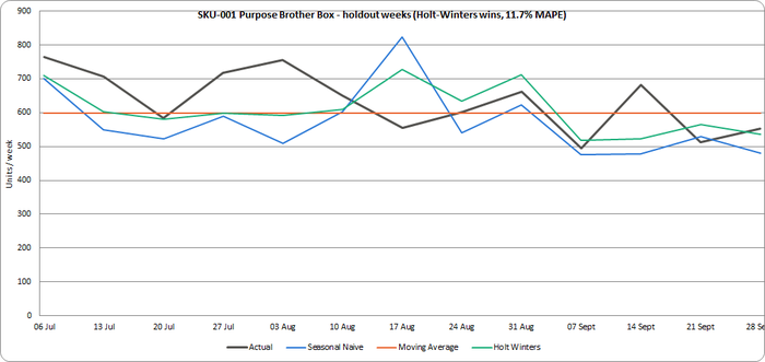
The winner is the method that matches the product’s behaviour, not the cleverest one. SKU-025 (Source Great Set) tops the table with a 5.0% MAPE from the moving average, while Holt-Winters managed only 24.3% and the seasonal naive 18.9%. The product’s demand had stepped down over the past year — the moving average of the last eight weeks followed it down, while both seasonal methods kept forecasting last year’s higher level and over-shot by 20–34 units a week. SKU-001 (Purpose Brother Box), by contrast, the second-largest seller at 508 units a week, has a clear seasonal pattern and Holt-Winters tracked it to 11.7%, beating the moving average (12.4%) and the seasonal naive (16.4%):

The moving average has a specific failure mode, and the table shows it. SKU-030 (Everything Surface Bag) posts a 109.6% MAPE for the moving average against 25.1% for the seasonal naive. The eight-week window just before the holdout contained a single promotion week of 534 units, three times the normal level; the moving average absorbed it and forecast a flat 231 units a week into a quarter in which demand slid from 161 to 82. Its bias — +106 units a week — would have meant ordering nearly twice what was needed for three months. The seasonal naive, which simply looked at the same weeks a year earlier, followed the slide and finished the quarter with a bias of just +3 units a week.

A good MAPE can hide a bias. SKU-020 (According Song Box) is in the Moderate band with a respectable 15.4% MAPE from the moving average, yet its bias is −17.9%: the forecast ran consistently below actual sales. The chart shows why:

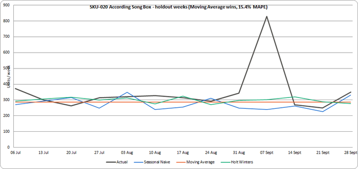
Twelve of the thirteen weeks are forecast to within a few dozen units; the week of 7 September was a promotion that sold 830 units against a forecast of 287, and that one week drags the whole quarter’s bias negative. Whether that counts as a forecasting failure depends on whether the promotion was planned: if it was, the forecast should have been overridden for that week by whoever planned it. Across the whole holdout, the 20 promotion weeks were forecast with an average error of 48.7%, against 25.1% for ordinary weeks — which is the single best argument for keeping the promotion calendar next to the forecast.

The bias column is the one to read before ordering. SKU-012 (Mouth Play Tin) has a 28.2% MAPE and a bias of +22.4%: the moving average would have over-ordered it by more than a fifth every week of the quarter. SKU-022 (Save Knowledge Set) is the mirror image at −24.3% — a stockout waiting to happen. Both would look acceptable if you only read the MAPE.

From forecast error to safety stock: the number that saves money

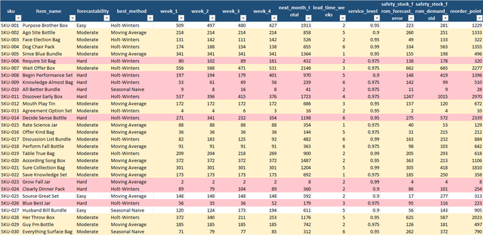
This is the tab that connects back to the inventory control post. For each SKU the winning method is re-fitted on the full three years and produces the next four weeks — 22,373 units across the 30 SKUs, roughly €1.02 million at list price. Then two safety stocks are computed side by side, both with the SKU’s own lead time and target service level:

• Safety stock from forecast error — z × RMSE of the winning forecast × √lead time. This is the buffer you need against the part of demand the forecast can’t explain.
• Safety stock from demand std. dev. — z × standard deviation of weekly demand × √lead time. This is the buffer you need if you ignore the forecast and treat every week-to-week swing, including the predictable seasonal ones, as risk. It is what the classic reorder-point formula uses when nobody has a forecast.

Across all 30 SKUs the forecast-based safety stock is 6,464 units against 8,065 — 1,601 fewer units, a 19.9% reduction, worth about €46,000 less inventory at list price (€328k against €374k). But the average hides where the saving actually comes from:

Forecastability	Safety stock from forecast error	Safety stock from demand std. dev.	Reduction
Easy (3 SKUs)	296 units (€14.7k)	701 units (€23.4k)	−58%
Moderate (18 SKUs)	4,022 units (€192.7k)	4,851 units (€220.6k)	−17%
Hard (9 SKUs)	2,146 units (€120.7k)	2,513 units (€130.0k)	−15%

The Easy products more than halve their buffer. SKU-025, the table-topper, needs 17 units of safety stock against 277 from the raw-variability formula — because its apparent volatility (a coefficient of variation of 0.71) was almost entirely the predictable step-down that the moving average followed. SKU-016 (Offer Kind Bag) drops from 215 to 31. SKU-014 (Decide Sense Bottle), a Hard SKU with a 61.9% MAPE, still halves its buffer from 572 to 275, because even a rough seasonal forecast explains a lot of a strongly seasonal product’s swing.

And then there are the seven SKUs where the forecast-based safety stock is higher — where the forecast error on the holdout was larger than the raw variability of demand. The largest is SKU-011 (Discover Early Box), the biggest seller in the range at 532 units a week:

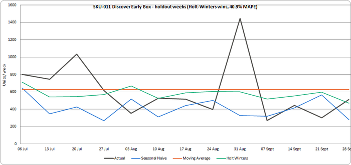
Two spikes in the quarter — 1,033 units in the week of 20 July and a flagged promotion week of 1,448 at the end of August — against ordinary weeks of 300 to 500, and a slump to 268 the week after the promotion. Holt-Winters “won” with a 40.9% MAPE, but its RMSE of 318 units implies 1,247 units of safety stock against 1,015 from the plain formula. That is not a reason to distrust forecasting; it is the workbook telling you, honestly, that this product’s demand is driven by something the sales history alone can’t see — the promotion calendar, and whatever caused the July spike — and that until that is fed in, the forecast is not buying you any inventory reduction on this SKU. The three lumpy movers (SKU-010, SKU-013, SKU-023, each selling under 10 units a week) sit in the same category for a different reason: with up to 16.7% of weeks at zero sales, a percentage error is close to meaningless, and these products need an intermittent-demand method or a simple min/max rule rather than a weekly forecast.

The business impact, in real numbers

Put a cost on what the workbook found:

1. Picking the method per product beats picking one method for everything. 26.3% average error against 32.3% for the best single method. On 22,000 units a month, that six-point gap is roughly 1,300 units a month ordered wrongly in one direction or the other.
2. About €46,000 of safety stock, one-eighth of the buffer, can come out simply by sizing it against forecast error rather than raw variability — and on the Easy products the buffer more than halves. That is working capital the previous post priced at the company’s cost of capital, released without touching service levels.
3. Three products would have been systematically over-ordered by about a fifth every week, and four under-ordered by a fifth to a half — visible only in the bias column. Catching one of those before Q4 ordering pays for the whole exercise.
4. Promotion weeks were forecast twice as badly as ordinary weeks (48.7% against 25.1%). A sales history knows nothing about next month’s promotion; the person who planned it does. The forecast tells you exactly how much that person’s input is worth.
5. The data-quality dividend. 2% of the raw rows were unusable, and the validator’s report says which, and why, and how many weeks per SKU had to be interpolated as a result. A forecast quietly built on a series with a −45 in it is worse than no forecast.

What to actually do with this, this week

1. Export weekly sales by SKU for the last two to three years from your point-of-sale, ERP or invoicing system: SKU, week, units sold. That is the entire data requirement. If you can add a flag for weeks the product was on promotion, do — it is the single most useful extra column. Holt-Winters needs at least two full years to learn a seasonal pattern; with less, use the moving average and seasonal naive and revisit next year.
2. Hold back the last quarter and score before you trust. Never judge a method on how well it fits the past; judge it on how well it forecast a period it hadn’t seen. The pipeline below does this automatically.
3. Start with the Forecastability tab, then the bias column. If most of your volume is Easy or Moderate, a simple method is good enough for Q4 ordering. Then read the bias column for every SKU you’re about to order and adjust the ones that are systematically off.
4. Recompute safety stock from forecast error, and compare it with what you hold today. Where the forecast-based number is lower, that is stock you can stop replacing. Where it is higher, ask what the forecast is missing — almost always promotions or a customer whose orders are lumpy — and get that information into the process.
5. Re-run it monthly. Roll the window forward, re-score, and watch whether each SKU’s winner and error stay stable. A product whose best method flips every month is telling you its behaviour is changing.

Try it yourself: a demo you can run in minutes

To make this concrete, simple-demand-forecasting is a small, self-contained, open-source Python pipeline. It:

1. Generates a fake SKU master (name, category, price, lead time, target service level) and three years of weekly unit sales per SKU with trend, seasonality, an optional Q4 peak, promotion weeks and noise baked in, plus a configurable share of deliberately corrupted rows.
2. Validates every row of both files against a strict schema, drops duplicates and sales for SKUs that don’t exist in the master, and writes a rejection report with a reason for every dropped row.
3. Rebuilds a gap-free weekly series per SKU, holds back the last 13 weeks, fits and scores the seasonal naive, moving average and Holt-Winters methods, picks a winner per SKU, re-fits it on the full history for the next four weeks, and writes it all into a single 7-tab Excel workbook — including the safety stock and reorder point each forecast implies.

Downloading the code (no Git experience needed)

You don’t need to know Git or the command line to get the code onto your computer:

1. Go to the repository: github.com/MattProtopapas/simple-demand-forecasting
2. Click the green <> Code button near the top of the page.
3. Click “Download ZIP” in the dropdown.
4. Right-click the downloaded ZIP and choose “Extract All…“ to unzip it into a regular folder.
5. Open that folder — that’s the project. Ask your AI tool of choice (I used Claude) to set up a Python environment and install the dependencies listed in requirements.txt — no coding experience required to get it running.

If you’re comfortable with Git, git clone https://github.com/MattProtopapas/simple-demand-forecasting.git does the same thing in one step.

Running the demo

The repository includes a full README.md, but the short version, from PowerShell (requires Python 3.10+; no pandas, numpy or statsmodels needed — every method is plain standard-library Python, so you can read exactly what Holt-Winters is doing):

python -m venv .venv
.\.venv\Scripts\Activate.ps1
pip install -r requirements.txt

python generate_data.py --skus 30 --weeks 156 --error-rate 0.02 --seed 42   # step 1: fake SKU master + weekly sales
python validate_data.py                                                     # step 2: schema checks, rejection report
python forecast_demand.py                                                   # step 3: three methods -> 7-tab Excel workbook

Then open output/demand_forecast.xlsx. With --seed 42 you’ll get exactly the numbers quoted in this post; the workbook committed to the repository was produced the same way, so you can also just browse it on GitHub without running anything. (One caveat: the generator dates the history to end on the most recent Monday, so if you run it later than the week this post was written the weeks will be labelled differently — the demand pattern and every score will be the same.)

Options worth playing with: --skus and --weeks change the size of the dataset; --error-rate 0 gives a perfectly clean dataset (and an empty validation report); a different --seed gives a different set of products and a different story. Four settings live in forecast_common.py rather than on the command line, because they are policy rather than parameters: HOLDOUT_WEEKS (13 — how much history to hold back for scoring), FORECAST_HORIZON_WEEKS (4 — how far ahead “next month” is), MOVING_AVERAGE_WINDOW (8 — try 4 and 13 and watch which SKUs change hands), and the FORECASTABILITY_BANDS (15% and 30% — the thresholds are a judgement, not a law).

Every input and output path is defined in one place in forecast_common.py, so once you’re comfortable with the demo you can drop your own real weekly sales and SKU master — matching the column layouts there — into data/, skip generate_data.py entirely, and run validate_data.py and forecast_demand.py straight on your own products.

Note: the sample data shipped with this repo is synthetic and randomly generated, and this project is intended for educational and demonstration purposes only — see the repository’s Disclaimer & EULA for details. It’s a starting point for understanding how demand forecasting and forecast accuracy measurement work, not a production planning system.

Understanding the results

The workbook — output/demand_forecast.xlsx — has seven tabs, in the order you should read them.

The inputs (two tabs). Input Data is the validated weekly sales, exactly as the forecasts read them — one row per SKU per week, with the units sold and the promotion flag. SKU Master holds the static attributes: name, category, unit price, lead time in weeks and target service level. The last two are what the safety-stock calculation uses. Alongside these, data/validation_report.txt lists every rejected row and why.

The scorecard. Accuracy League Table — one row per SKU, ranked by the winning method’s MAPE, with each method’s MAE, MAPE and bias side by side, the winner, its bias as a percentage of demand, the SKU’s average weekly demand and coefficient of variation over the last year, the share of zero-sales weeks (the lumpy-mover warning), and the number of weeks the validator had to fill in. Moderate rows are shaded yellow, Hard rows red. Forecastability is the roll-up: SKU count, share of volume and average error per band, and how often each method won.

The evidence. Forecast vs Actual is every holdout week for every SKU — 390 rows — with the actual, all three forecasts, the winner’s error and its percentage error:

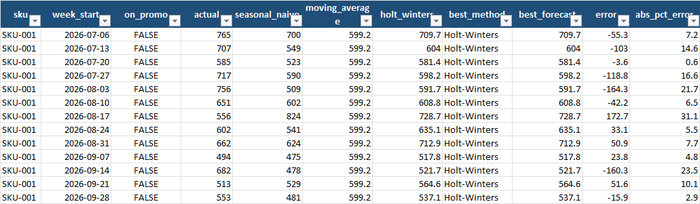
This is the tab to open when a league-table number looks odd. It is where you can see that SKU-030’s moving average forecast 231 units a week into weeks that sold 80, or that SKU-020’s whole quarter is one promotion week. The Charts tab draws the same thing for the six highest-volume SKUs, with the actual in dark grey and each method in a consistent colour.

The decision. Next Month Forecast — the winning method re-fitted on the full history, the next four weeks and their total, the forecast’s RMSE, the safety stock it implies next to the safety stock the raw-variability formula implies, the expected demand over the lead time, and the resulting reorder point. It is the one tab to hand to whoever places the orders.

The limits worth keeping in mind

Demand forecasting, like every tool covered on this blog, is genuinely useful within real limits:

• The forecast only knows what the history knows. A new product, a lost customer, a competitor’s opening, or next month’s promotion are invisible to every method here. The right use of the forecast is as the baseline that a human adjusts for the things they know and the data doesn’t — and the promotion-week error (48.7% against 25.1%) is a measure of how much that adjustment is worth.
• One holdout quarter is one sample. Thirteen weeks is enough to tell Easy from Hard and to catch a gross bias; it is not enough to be sure that a 15.4% MAPE is really better than a 16.2% one. Re-run monthly and watch for stability rather than trusting any single ranking.
• MAPE breaks on small numbers. A product that sells two units a week and is forecast at three has a 50% error. For the lumpy movers, read MAE (units) and the share of zero weeks, and use a min/max rule or an intermittent-demand method rather than a weekly forecast.
• Holt-Winters needs two full seasons. With less than 104 weeks of history it falls back to the moving average — and even with three years, a 52-week seasonal pattern is being learned from three examples of each week. Treat its seasonal shape as approximate.
• Safety stock from forecast error assumes the error is roughly normal and stable. Promotion spikes are neither. Where the forecast-based buffer comes out higher than the raw-variability one, that is the assumption failing, and the fix is better inputs, not a bigger buffer.
• The demo’s lead times and service levels are illustrative. Real ones come from your suppliers and your customers’ tolerance for a stockout — the inventory control post covers how to set them.

None of that diminishes the core value. The sales history already exists in your systems. The methods have been standard for more than half a century — Charles Holt published his in 1957 and Peter Winters added the seasonal term in 1960. What forecasting changes is not that you know the future, but that you know how well you know it, product by product — and that, rather than the forecast itself, is what tells you how much stock to hold, which products to watch, and where a person’s judgement is worth more than any method.

← Back to all posts